Time Series Example
Before a time series calculation can take place, a pandapipes network must be created.
This can be created by yourself as described in Creating a Network
or loaded from the existing Networks via pandapipes.networks.<network name/ path>.
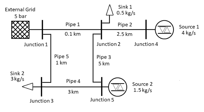
In this case the following simple water network is created:
import pandapipes

# create empty network
net = pandapipes.create_empty_network("net", add_stdtypes=False)

# create fluid
pandapipes.create_fluid_from_lib(net, "water", overwrite=True)

# diameter for the pipes
d = 75e-3

# create junctions
j0 = pandapipes.create_junction(net, pn_bar=5, tfluid_k=293.15, name="Junction 1")
j1 = pandapipes.create_junction(net, pn_bar=5, tfluid_k=293.15, name="Junction 2")
j2 = pandapipes.create_junction(net, pn_bar=5, tfluid_k=293.15, name="Junction 3")
j3 = pandapipes.create_junction(net, pn_bar=5, tfluid_k=293.15, name="Junction 4")
j4 = pandapipes.create_junction(net, pn_bar=5, tfluid_k=293.15, name="Junction 5")

# create external grid
pandapipes.create_ext_grid(net, j0, p_bar=5, type="pt", t_k=293.15, name="External Grid")

# create sinks
pandapipes.create_sink(net, j1, mdot_kg_per_s=0.5, name="Sink 1")
pandapipes.create_sink(net, j2, mdot_kg_per_s=3, name="Sink 2")

# create sources
pandapipes.create_source(net, j3, mdot_kg_per_s=4, name="Source 1")
pandapipes.create_source(net, j4, mdot_kg_per_s=1.5, name="Source 2")

# create pipes
pandapipes.create_pipe_from_parameters(net, j0, j1, length_km=0.1, diameter_m=d, k_mm=0.1, name="Pipe 1")
pandapipes.create_pipe_from_parameters(net, j1, j3, length_km=2.5, diameter_m=d, k_mm=0.2, name="Pipe 2")
pandapipes.create_pipe_from_parameters(net, j1, j4, length_km=5, diameter_m=d, k_mm=0.05, name="Pipe 3")
pandapipes.create_pipe_from_parameters(net, j4, j2, length_km=3, diameter_m=d, k_mm=0.3, name="Pipe 4")
pandapipes.create_pipe_from_parameters(net, j0, j2, length_km=1, diameter_m=d, k_mm=0.35, name="Pipe 5")
Then the network must be prepared. Here the time series for the occurring sinks and sources of the network must be given. As in a steady-state calculation, the mass flows must be specified, whereby the number of mass flows corresponds to the number T of time steps. The mass flows for N sinks have to be written into a csv file as follows:
0 |
1 |
— |
sinkN-1 |
sinkN |
|
0 |
mass_flow_0_0 |
mass_flow_0_1 |
— |
mass_flow_0_N-1 |
mass_flow_0_N |
1 |
mass_flow_1_0 |
mass_flow_1_1 |
— |
mass_flow_1_N-1 |
mass_flow_1_N |
2 |
mass_flow_2_0 |
mass_flow_2_1 |
— |
mass_flow_2_N-1 |
mass_flow_2_N |
— |
— |
— |
— |
— |
— |
T-1 |
mass_flow_T-1_0 |
mass_flow_T-1_1 |
— |
mass_flow_T-1_N-1 |
mass_flow_T-1_N-1 |
T |
mass_flow_T_0 |
mass_flow_T_1 |
— |
mass_flow_T_N-1 |
mass_flow_T_N |
For this network, the structure of the csv files for the sinks and sources must look like this:
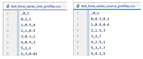
The corresponding csv file is afterwards read out and the resulting DataFrames are
then written into the network with the help of the controller ConstControl.
Now a variable time_steps can be defined, which contains integer steps
from 0 to T, in the example T is equal to 6. The prepared network and time_steps
are needed to create an OutputWriter ow.
This later contains the results of the time series simulation.
Finally, the main function for starting the simulation can be called.
run_timeseries_ppipe(net, time_steps, output_writer=ow) contains the
time loop in which the run_control function of pandapower is nested,
see Time Series Module Overview.
In the following the code for the previous descriptions is listed:
import os
import pandas as pd
import pandapower.control as control
import pandapipes
from pandapower.timeseries import DFData
from pandapower.timeseries import OutputWriter
from pandapipes.timeseries import run_timeseries_ppipe
from pandapipes import pp_dir

# prepare grid
profiles_sink = pd.read_csv(os.path.join(pp_dir, 'test', 'pipeflow_internals', 'data',
                                         'test_time_series_sink_profiles.csv'), index_col=0)
profiles_source = pd.read_csv(os.path.join(pp_dir, 'test', 'pipeflow_internals', 'data',
                                           'test_time_series_source_profiles.csv'), index_col=0)
ds_sink = DFData(profiles_sink)
ds_source = DFData(profiles_source)

const_sink = control.ConstControl(net, element='sink', variable='mdot_kg_per_s',
                                  element_index=net.sink.index.values, data_source=ds_sink,
                                  profile_name=net.sink.index.values.astype(str))
const_source = control.ConstControl(net, element='source', variable='mdot_kg_per_s',
                                    element_index=net.source.index.values,
                                    data_source=ds_source,
                                    profile_name=net.source.index.values.astype(str))
del const_sink.initial_powerflow
const_sink.initial_pipeflow = False
del const_source.initial_powerflow
const_source.initial_pipeflow = False

# define time steps
time_steps = range(7)

# create OutputWriter
log_variables = [
    ('res_junction', 'p_bar'), ('res_pipe', 'v_mean_m_per_s'),
    ('res_pipe', 'reynolds'), ('res_pipe', 'lambda'),
    ('res_sink', 'mdot_kg_per_s'), ('res_source', 'mdot_kg_per_s'),
    ('res_ext_grid', 'mdot_kg_per_s')]
ow = OutputWriter(net, time_steps, output_path=None, log_variables=log_variables)

# run
run_timeseries_ppipe(net, time_steps, output_writer=ow)
Furthermore, the results of the simulation are accessible
via the OutputWriter ow and can be displayed with the print command:
print(ow.np_results["res_junction.p_bar"])
print(ow.np_results["res_pipe.v_mean_m_per_s"])
print(ow.np_results["res_pipe.reynolds"])
print(ow.np_results["res_pipe.lambda"])
print(ow.np_results["res_sink.mdot_kg_per_s"])
print(ow.np_results["res_source.mdot_kg_per_s"])
print(ow.np_results["res_ext_grid.mdot_kg_per_s"])